How to Health Science in R - Fisher’s Exact Test

Introduction

Fisher’s exact test is an independent test used to determine if there is a relationship between categorical (non-parametric) variables with a small sample size.
Used to assess whether proportions of one variable are different among values of another table.
Uses (hypergeometric) marginal distribution to derive exact p-values which are not approximated which are somewhat conservative.
The rules of Chi distribution do not apply when the frequency count is <5 for more than 20% of the cells in a contingency table (Bower 2003).
Data is easily manipulated by using a contingency table.

Assumptions

Assumes that the individual observations are independent.
Assumes that the row and column totals are fixed or conditioned.
The variables are categorical and randomly sampled.
Observations are count data.

Hypotheses

The hypotheses of Fisher’s exact test are similar to Chi-square test:

Null hypothesis:(H_0) There is no relationship between the categorical variables, the variables are independent.

Alternative hypothesis: (H_1) There is a relationship between the categorical variables, the variables are dependent.

Fisher’s Exact Test Equation

Fisher’s exact test for a one-tailed p-value is calculated using the following formula:

p = {(a+b)!(c+d)!(a+c)!(b+d)! \over a! b! c! d! n!} - n = population size/ total frequency - a + b = “successes” values in the contingency table - a + c = sample size / draws from the population - a = sample successes

Formula description

this test is usually used as a one-tailed test but it can also be used as a two tailed test as well, a,b,c, and d are the individual frequencies on the 2x2 contingency table and n is our total frequency. This particular test is used to obtain the probability of the combination of frequencies that we can actually obtain.

What is a contingency table?

This is a table that shows the distribution of a variable in the rows and columns. Sometimes referred to as a 2x2 table. They are useful in summarizing categorical variables. The table() function is used to create a contingency table in R. When the variables of interest are summarized in a contingency table it is easier to run the Fisher’s Exact test.

Example: Creating a contingency table

Lets say we have information on the gender of participants in a clinical trial and the type of drug administered to them we can create the following contingency table for further analysis.

Code

# Example R code to create a contingency table

# Creating a data frame
 df = data.frame (
   "Drug" = c("Drug A", "Drug B", "Drug A"),
   "Gender" = c("Male", "Male", "Female")
 )
 
# Creating contingency table using table()
 ctable = table(df)
 print(ctable)

        Gender
Drug     Female Male
  Drug A      1    1
  Drug B      0    1

Performing Fisher’s Exact Test in R

We will need to install the ggstatplot package to visualize the statistical results.

Code

#install.packages("ggstatplot") 
#install.packages("summarytools")
#install.packages("gmodels")
#install.packages("gt")
#install.packages("tidyverse")

Data Source: GMP2017

For this example we will be using the Greater Manchester Police’s UK stop and search data from 2017(December) sourced from the Sage Research Methods Dataset Part 2. This data has information on stop and search events, gender and ethnicity. For this example we would like to access whether there is a significant relationship between gender and stop and search events?

Code

GMP17 <- read.csv("dataset-gmss-2017-subset1.csv")

Load in libraries

Code

library(gmodels)
library(ggstatsplot)
library(gt)
library(gtsummary)
library(katex)
library(tidyverse)

Descriptive summary

head(GMP17)

  Gender Ethnicity ObjectSearch
1      1         1            1
2      1         1           -9
3      1         1            1
4      1         1            1
5      1         1           -9
6      1         1            1

str(GMP17)

'data.frame':   186 obs. of  3 variables:
 $ Gender      : int  1 1 1 1 1 1 1 1 1 -9 ...
 $ Ethnicity   : int  1 1 1 1 1 1 2 1 1 1 ...
 $ ObjectSearch: int  1 -9 1 1 -9 1 1 1 -9 -9 ...

# determining the number of rows
NROW(GMP17)

[1] 186

Assessing frequencies to answer research question

For this analysis we will use the Gender variable and the ObjectSearch variable

Code

# Dropping the Ethnicity variable to remain with variables of interest for for the 2x2 table

newGMP17 <-GMP17[ -c(2) ]
 
head(newGMP17)

  Gender ObjectSearch
1      1            1
2      1           -9
3      1            1
4      1            1
5      1           -9
6      1            1

The data contains missing values categorized as -9 that we need to drop and we need to rename our variables based on the data dictionary provided https://methods.sagepub.com/dataset/fishers-exact-gmss-2017-r.

Code

# Exclude rows that have missing data in both variables
newGMP17_nom <- subset(newGMP17, Gender > 0)
newGMP17_nom2 <- subset(newGMP17_nom, ObjectSearch  > 0)
summary(newGMP17_nom2)

     Gender       ObjectSearch  
 Min.   :1.000   Min.   :1.000  
 1st Qu.:1.000   1st Qu.:1.000  
 Median :1.000   Median :1.000  
 Mean   :1.052   Mean   :1.259  
 3rd Qu.:1.000   3rd Qu.:2.000  
 Max.   :2.000   Max.   :2.000

Code

nrow(newGMP17_nom2)

[1] 116

Code

# Renaming the Gender variable based on data dictionary
newGMP17_nom2$Gender <- 
  recode_factor(
    newGMP17_nom2$Gender,
            "1" = "Male",
            "2" = "Female"
)

# Renaming the Gender variable based on data dictionary
newGMP17_nom2$ObjectSearch <- 
  recode_factor(
    newGMP17_nom2$ObjectSearch,
            "1" = "Controlled_Drugs",
            "2" = "Harmful_Objects"
)

Code

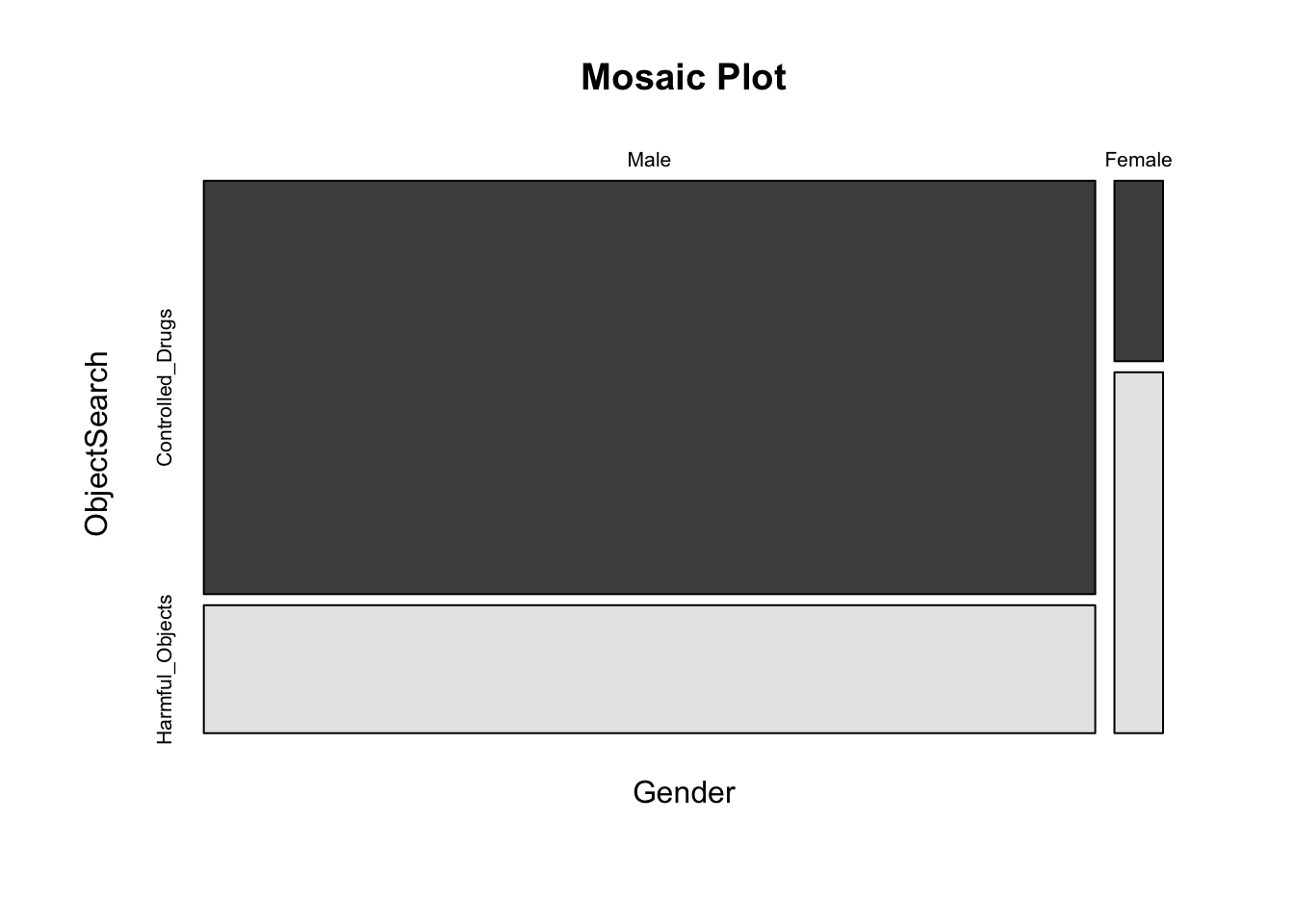
# Creating the contingency table for subset data
cGMP17 = table(newGMP17_nom2)
print(cGMP17)

        ObjectSearch
Gender   Controlled_Drugs Harmful_Objects
  Male                 84              26
  Female                2               4

Visualizing data using mosaic plot

we can use the mosaic plot to represent the data.

Code

mosaicplot(cGMP17,
           main ='Mosaic Plot',
           color = TRUE)

Running the Fisher’s exact test using fisher.test()

What if we just run a Chi-square test?

Using our GMP17 dataset we can try to run a Chi-square test instead of the Fisher’s Exact test and see what happens.

The R output gives us a warning that the Chi Square is not appropriate hence we should use another test in this case the Fisher’s Exact Test.

Code

chisq.test(cGMP17)$expected

Warning in chisq.test(cGMP17): Chi-squared approximation may be incorrect

        ObjectSearch
Gender   Controlled_Drugs Harmful_Objects
  Male          81.551724       28.448276
  Female         4.448276        1.551724

Running the test

Code

# running the fisher's exact test

test <- fisher.test(cGMP17)
test


    Fisher's Exact Test for Count Data

data:  cGMP17
p-value = 0.03809
alternative hypothesis: true odds ratio is not equal to 1
95 percent confidence interval:
  0.8528079 73.5937611
sample estimates:
odds ratio 
  6.331977

Using the gt summary to view results.

Code

newGMP17_nom2 |> 
  tbl_summary(by = Gender) |> 
   add_p() |> 
  add_overall()

Characteristic	Overall, N = 116¹	Male, N = 110¹	Female, N = 6¹	p-value²
ObjectSearch				0.038
Controlled_Drugs	86 (74%)	84 (76%)	2 (33%)
Harmful_Objects	30 (26%)	26 (24%)	4 (67%)
¹ n (%)
² Fisher’s exact test

Interpretation of results

The most important test statistic is the p - value therefore we can retrieve the specific result using the following code;

Code

test$p.value

[1] 0.03808788

Odds ratio = 6.33, 95% CI = 0.85-73.59], we reject the null hypothesis (p < 0.05) and conclude that there is a strong association between the two categorical independent variables (gender and object search events)

Therefore the odds ratio indicates that the odds of getting stopped and searched by gender is 6.33 times as likely for males compared to females. In other words, males are more likely of getting stopped and searched than females.

Visualizing statistical results with plots using ggstatsplot

we download the ggsattsplot package to visualize the results in a plot.

Code

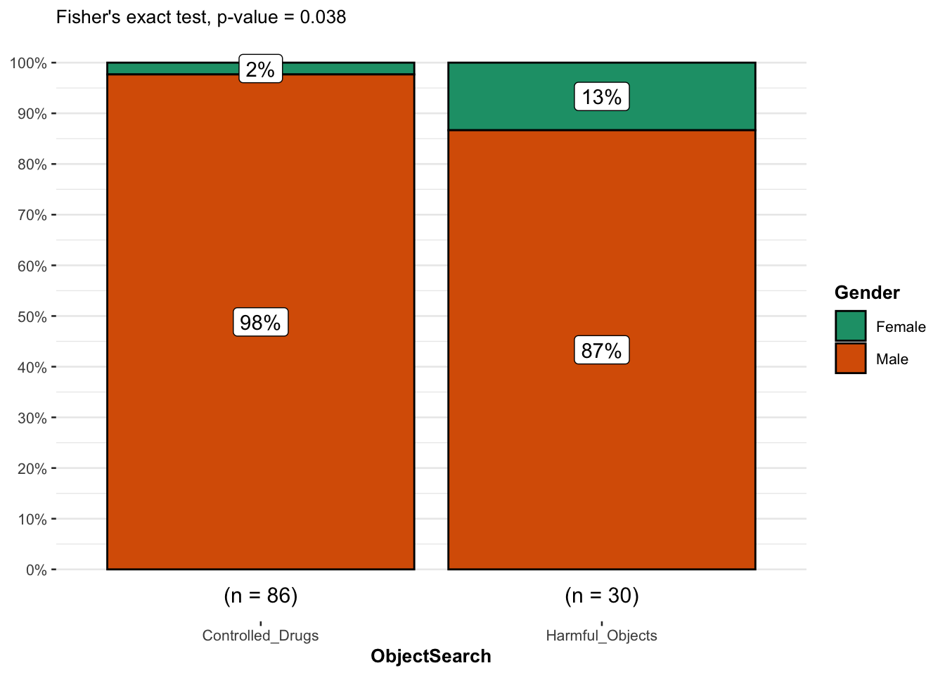
# Fisher's exact test 

test <- fisher.test(cGMP17)

# combine plot and statistical test with ggbarstats

ggbarstats(
 newGMP17_nom2, Gender, ObjectSearch,
 results.subtitle = FALSE,
 subtitle = paste0(
 "Fisher's exact test", ", p-value = ",
 ifelse(test$p.value < 0.001, "< 0.001", round(test$p.value, 3))
  )
 )

From the plot, it is clear that the proportion of males among object search events is higher compared to females, suggesting that there is a relationship between the two variables.

This is confirmed thanks to the p-value displayed in the subtitle of the plot. As previously, we reject the null hypothesis and we conclude that the variables gender and stop and search events are not dependent (p-value = 0.038).

What if we have more than two levels?

Using the drug example used previously lets say we have 3 drugs ‘Drug A, Drug B or Drug C’ and we want to see if there is any relationship with gender ‘Male/Female’.

Code

# Creating a data frame
 df = data.frame (
   "Drug" = c("Drug A", "Drug B", "Drug A", "Drug C", "Drug C"),
   "Gender" = c("Male", "Male", "Female", "Female", "Female")
 )
 
# Creating contingency table using table()
 ctable = table(df)
 print(ctable)

        Gender
Drug     Female Male
  Drug A      1    1
  Drug B      0    1
  Drug C      2    0

Code

# Running the Fisher's Exact test for the 3x2 table
fisher.test(ctable)


    Fisher's Exact Test for Count Data

data:  ctable
p-value = 0.6
alternative hypothesis: two.sided

The p-value is non-significant [p = 0.6], we fail to reject the null hypothesis (p < 0.05) and conclude that there is no association between the drug treatments and gender. If the results had been significant we would have gone ahead and conducted a pair wise comparison.

References

Bower, Keith M. 2003. “When to Use Fisher’s Exact Test.” In American Society for Quality, Six Sigma Forum Magazine, 2:35–37. 4.
McCrum-Gardner, Evie. 2008. “Which Is the Correct Statistical Test to Use?” British Journal of Oral and Maxillofacial Surgery 46 (1): 38–41.
Wong KC. Chi squared test versus Fisher’s exact test. Hong Kong Med J. 2011 Oct;17(5):427
Patil, I. (2021). Visualizations with statistical details: The ‘ggstatsplot’ approach. Journal of Open Source Software, 6(61), 3167, doi:10.21105/joss.03167
Zach Bobbit. (2021). Fisher’s Exact Test: Definition, Formula, and Example
Bobbitt, Z. (2020). “Fisher’s Exact Test: Definition, Formula, and Example.” statology.org